한국 등록농약 피부투과 물성공간의 군집부재 진단과 space-filling 기반 대표 물질 선정

서    론

농약 원제(active ingredient)는 인체에 여러 경로로 노출되며, 농작업자의 경우 경피 노출이 주된 경로로 알려져 있다(Krieger, 1995). 이에 따라 피부에 부착된 양 중 실제로 체내에 흡수되는 비율, 즉 피부흡수율은 농작업자 위해성 평가의 핵심 입력값으로 사용된다(EFSA, 2017; OECD, 2004).

피부흡수율의 표준 산출법은 OECD 시험지침 428(in vitro 피부흡수 시험)에 규정되어 있지만, 고비용 및 전문인력과 시설이 필요하다는 한계가 있다. 이러한 제약으로 규제 현장에서는 실측값 대신 기본값이 널리 사용된다(EFSA, 2017; RDA, 2026). 국내에서는 단일 기본값을 일률적으로 적용하는 반면, 유럽식품안전청(European Food Safety Authority, EFSA)은 제형에 따라 기본값을 적용하고 있다(EFSA, 2017). 또한 옥탄올-물 분배계수(log P)와 분자량(molecular weight, MW)의 기준으로 기본값을 구분 적용하는 방식도 사용되어 왔으며, 국내에서도 이 기준에 따라 유효성분의 기본값을 분류하고 노출량을 산출한 사례가 보고되었다(You et al., 2017). 그러나 일률적 기본값과 이분법적 임계값은 물질 간 물성 차이를 충분히 반영하지 못하므로 화학물질별 예측하는 방향으로 전환이 요구된다.

이러한 요구에 대응하여 컴퓨팅 기술(in silico) 기반 대체시험법이 그 대안으로 관심을 받아왔다. 다만 예측모델 개발에는 학습 및 검증용 실측 자료가 필연적으로 요구되는데, 국내에 등록된 수백 종의 농약 원제 전체를 실측하는 것은 현실적으로 불가능하다. 따라서 어떤 물질을 우선 측정할 것인가라는 선정 문제가 모델 개발에 선행한다. 선정이 편향되면 학습 및 검증 자료 자체가 물성 스펙트럼의 일부에만 치우치게 되므로, 이는 모델링에 앞서 해결되어야 할 설계 문제이다(Daszykowski et al., 2002). 한편 최근 농약 및 화학물질 연구에서는 실측값 없이 물리화학·구조 정보만으로 화학 공간을 특성화하고 이를 근거로 시험 대상을 선정하는 흐름이 나타나고 있다(Kar et al., 2025; Renai et al., 2025).

그런데 실측 자원의 배분 방식은 물성 공간의 구조에 따라 달라진다. 공간이 서로 구분되는 군집으로 이루어져 있다면 각 군집의 대표를 뽑는 분류 기반 선정이 타당하고(Golbraikh and Tropsha, 2002), 경계 없는 연속체라면 공간 전체를 고르게 덮는 space-filling 설계가 타당하다(Kennard and Stone, 1969). 이때 분류 기반 선정은 공간에 군집이 실재한다는 것을 전제로 하지만, 군집화 알고리즘은 구조가 없는 자료에서도 분할을 산출하므로 사전에 자료의 구조를 확인하지 않으면 얻어진 군집이 자료의 성질인지 알고리즘의 산물인지 구별할 수 없다(Adolfsson et al., 2019). 한편 space-filling 설계는 한정된 표본을 물성 공간에 고르게 배치함으로써 대표성을 확보하며, 이러한 배치가 예측 신뢰도를 높인다는 점은 QSAR 분야에서 입증되었다(Martin et al., 2012). 두 전략 중 어느 쪽이 적절한지가 자료의 구조에 의존한다는 점은 지적된 바 있다(Daszykowski et al., 2002).

그럼에도 앞서의 연구들은 화학공간을 고르게 탐색한다는 방침만을 채택하였을 뿐, 해당 공간이 그 방침에 적합한 구조인지는 검정하지 않았다. 또한 국내 등록 농약 원제의 물성공간이 어떤 구조를 갖는지는 아직 보고된 바가 없다.

본 연구는 국내 등록 농약 원제의 물성공간에 군집 구조가 실재하는지를 진단하고, 그 결과에 부합하는 대표물질 선정 전략을 제시하는 것을 목적으로 한다. 군집 구조의 실재 판정(clusterability)에서는 단일 지표에 의존한 판정의 위험성이 지적되어 왔으므로(Adolfsson et al., 2019; Ronan et al., 2016), 원리가 서로 다른 복수의 진단을 교차 확인하였다. 또한 진단 절차 자체의 검정력를 양성 및 음성 대조군으로 검증하였으며, 선정 결과의 타당성은 무작위 선정 대비 커버리지로 확인하였다. 흡수율 실측값은 사용하지 않으며, 따라서 구조 진단과 그에 근거한 선정까지를 범위로 한다.

재료 및 방법

국내 등록 농약 원제의 물리화학 정보를 수집하여 분석 대상 집합을 구성하고, 물질을 물성 공간에 배열할 좌표축으로 피부투과계수를 산정하였다. 이어서 원리가 서로 다른 복수의 지표로 물성 공간의 군집 구조 실재 여부를 진단하였으며, 진단 절차 자체의 타당성은 인공 양성 및 음성 대조군으로 검증하였다. 판정된 구조 아래에서 보유 표본이 물성 공간을 충분히 덮는지를 정량화한 뒤, 대표 농약을 선정하고 무작위 선정과의 커버리지 대조로 그 타당성을 확인하였다(Fig. 1).

Fig. 1.

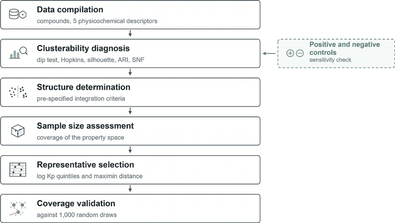
Study workflow for diagnosing the structure of the physicochemical property space and selecting representative compounds.

군집가능성 진단

물성 공간에 자연적인 군집 구조가 존재하는지를 원리가 서로 다른 다섯 가지 진단으로 평가하였다. 물성 공간은 다섯 개의 물성 변수로 정의하되, dip 검정은 1변량 검정이므로 다변량 적용 시 데이터를 1차원으로 축소한 뒤(제1주성분 및 두 점 사이 거리) 검정하였으며, 개별 물성 변수와 정렬 축 log Kp의 주변분포에 대한 dip은 보조 및 탐색 지표로만 산출하였다.

각 진단의 입력 뷰와 적용 대상은 Table 1과 같다. 단변량 및 저차원 진단(dip test, Hopkins, PCA, UMAP)은 5 물성 변수로 정의된 물성 뷰에 적용하였고(N = 356, 5변수 완전 보유 데이터), 다중뷰 융합(similarity network fusion, SNF)은 물성 뷰와 구조 뷰를 함께 사용하였다(N = 354).

Table 1.

Definition of the input views used for the clusterability diagnostics

Dip test of unimodality

각 변수의 주변분포가 단봉(unimodal)인지 다봉(multimodal)인지를 Hartigan and Hartigan (1985)의 dip 통계량으로 검정하였다(diptest 패키지). (i) 제1주성분에 투영한 값(PCA-dip)과 (ii) 모든 두 점 사이의 유클리드 거리 분포에 각각 dip을 적용하였다. 다변량 자료는 dip을 직접 적용할 수 없어 1차원으로 축소해야 하며, 점 간 거리 분포를 이용하는 방안은 Kalogeratos and Likas (2012)에서 착안하였으며, 모든 두 점 사이 거리를 하나의 분포로 모아 검정하는 방법을 따랐다(Adolfsson et al., 2019). 추가로 각 물성변수 및 log Kp의 주변분포에 대한 개별 dip도 산출하였다.

Hopkins

통계량 데이터의 군집화 경향(clustering tendency)을 Hopkins 통계량으로 평가하였다. 0.5는 균등 분포, 1에 가까울수록 비균등(non-uniform)을 의미한다. 무작위 표본 추출에 따른 변동을 줄이기 위해 시드 0-19의 20회 반복 평균을 사용하였다. 통계량 산출 시 최근접이웃거리는 데이터 차원수 d만큼 거듭제곱하여 합산하였다(Hopkins and Skellam, 1954; Wright, 2022).

차원 축소(PCA 및 UMAP)

표준화된 다차원 공간을 PCA와 UMAP(McInnes et al., 2018)으로 2차원에 투영하여 군집의 시각적 분리 여부를 확인하였다. UMAP이 만들어내는 인위적 군집 착시를 배제하기 위해 PCA 결과와 교차 확인하였다(Kobak and Linderman, 2021).

다중뷰 융합(SNF) 게이트

물성 정보만으로 드러나지 않는 군집이 분자 구조 정보를 함께 고려하면 나타나는지 확인하기 위해, 물성 뷰와 구조 뷰를 SNF(Wang et al., 2014)로 융합하였다. 물성 뷰는 5 물성 변수이며, 구조 뷰는 각 화합물의 Morgan/ECFP4 지문(2048-bit, radius 2)에서 산출한 Tanimoto 거리(1-유사도)를 입력으로 한다(뷰 정의는 Table 1). 이웃수 K, 커널 스케일 μ, 군집수 C의 모든 조합(총 180개 설정)을 클러스터링 하였다(Table 2). 탐색 범위는 Wang et al. (2014)의 권장(μ∈[0.3, 0.8]) 및 표본수 기반 이웃수 규칙(K ≈ N/20 ~ N/40)에 따라 설정하였고, 군집수 C는 과소 및 과대분할을 배제하기 위해 4−8로 사전 지정하였다. 각 설정의 군집 유효성은 군집이 형성된 본래 특성 공간에서 실루엣 계수(silhouette coefficient; Rousseeuw, 1987)로 평가하였다. 실루엣 임계값 0.25는 분석 전에 사전 고정(pre-specified)하였으며, 결과를 관찰한 뒤 조정하지 않았다. 다만 군집 존재 여부의 최종 판정의 임계값이 아니며, 대조군과의 상대 비교에 근거하여 판정하였다.

Table 2.

Hyperparameter search grid for the SNF fusion-network clustering

분석은 Python에서 수행하였으며, 분자 지문은 RDKit, SNF 융합은 snfpy, 실루엣 및 spectral clustering은 scikit-learn(Pedregosa et al., 2011)을 사용하였다.

그룹화 경계의 안전성(ARI)

물성 공간에 자연적 경계가 있다면 그룹화 방법을 바꾸어도 유사한 경계가 재현되어야 한다. log Kp를 기준으로 400종을 네 가지 방법(등간격 구간화, 분위 구간화, log Kp 1차원 k-means, log Kp·log P·MW의 3변수 k-means; 모두 k = 5)으로 5개 그룹으로 나눈 뒤, 방법 간 그룹 라벨의 일치도를 ARI(adjusted Rand index; Hubert and Arabie, 1985)로 산출하였다.

군집 존재 여부의 종합 판정은 단일 지표에 의존하지 않고, dip과 PCA/UMAP를 핵심 판별자로, Hopkins와 SNF를 보조 지표로 삼는 규칙을 분석 전에 정하였다.

결과 및 고찰

피부투과 물성 공간의 군집 부재

5개의 물성 변수로 정의한 국내 등록 농약 원제의 피부투과 물성 공간에서는 자연적인 군집 구조가 관찰되지 않았다. 다봉성 검정, 차원축소 시각화, 다중뷰 군집성 평가 및 그룹 일치도 분석의 네 가지 독립적인 진단은 모두 일관되게 군집 부재(clusterability absence)를 지지하였다.

먼저, 다변량 자료를 1차원으로 축소하여 수행한 다봉성 검정에서도 군집의 증거는 확인되지 않았다. 제1주성분에 대한 dip 검정(PCA-dip)과 두 점 사이 거리 기반 dip 검정(Dip-dist)은 모두 단봉 분포를 나타냈으며(각각 p = 0.965, p = 0.991), 개별 물성 변수의 주변분포 역시 모두 단봉으로 나타났다(p = 0.96−0.99). 특히 dip-dist는 좌표가 아닌 두 점 사이 거리를 이용하므로 투영 방향에 영향을 받지 않으며, 방향성과 무관한 군집성 검정으로 알려져 있다(Adolfsson et al., 2019; Kalogeratos and Likas, 2012). 따라서 축 선택이나 투영 방향에 관계없이 자료는 하나의 연속적인 분포를 형성하는 것으로 판단되었다.

차원축소 결과에서도 동일한 양상이 확인되었다(Figs. 2 and 3). PCA에서는 분리된 집단 없이 하나의 연속적인 점구름(point cloud)이 형성되었으며, 비선형 구조를 보존하는 UMAP에서도 명확한 군집이나 경계는 관찰되지 않았다. 즉, 선형 및 비선형 차원축소 모두에서 자료는 독립적인 하위 집단보다 연속적인 물성 스펙트럼의 형태를 나타냈다.

Fig. 2.

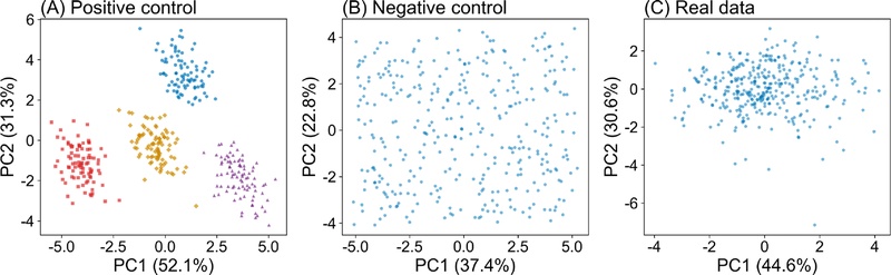
Two-dimensional principal component analysis (PCA) projections of the three datasets. (A) Positive control, four Gaussian clusters generated by make_blobs; (B) negative control, a uniform random distribution; (C) real data, 356 registered pesticides described by five physicochemical properties (log P, MW, melting point, water solubility, vapour pressure) after log transformation and z-score standardization. Axis labels indicate the percentage of variance explained by each principal component. In (A), colors and marker shapes denote the four generative clusters. All three datasets share the same sample size (N = 356), dimensionality (5), and were constructed over the same per-variable value range.

Fig. 3.

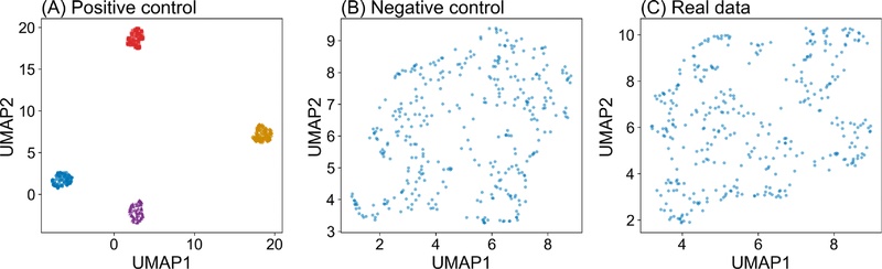
Two-dimensional UMAP projections of the three datasets. (A) Positive control, four Gaussian clusters generated by make_blobs; (B) negative control, a uniform random distribution; (C) real data, 356 registered pesticides described by five physicochemical properties after log transformation and z-score standardization. In (A), colors and marker shapes denote the four generative clusters. UMAP parameters: n_neighbors = 15, min_dist = 0.1. All three datasets share the same sample size (N = 356), dimensionality (5), and per-variable value range. UMAP axis coordinates are dimensionless and their absolute scale carries no direct interpretation.

반면 Hopkins 통계량은 0.951로 계산되어 자료가 물성 공간 전체에 균등하게 분포하지 않고 특정 영역에 집중되어 있음을 시사하였다. 그러나 Hopkins 통계량은 공간적 비균등성(spatial inhomogeneity)을 평가하는 지표로, 높은 값은 데이터가 균등하게 분포되어 있지 않음을 의미할 뿐 자연적인 군집의 존재를 직접 의미하지는 않는다. 따라서 본 결과는 물질이 일부 물성 영역에 밀집되어 있음을 보여주지만, 앞선 군집성 진단 결과와 모순되지는 않는다.

군집 부재가 선택한 5개의 물성 변수에 의존한 결과인지를 확인하기 위해 구조 지문(fingerprint)과 물성 정보를 결합한 SNF 기반 다중뷰 분석을 수행하였다. 사전에 설정한 실루엣 임계값(0.25)을 기준으로 180개의 매개변수 조합을 평가한 결과, 임계값을 만족한 경우는 없었다(0/180). 구조 뷰 단독의 최대 실루엣 계수는 0.042, 융합망에서는 0.035로 모두 기준값의 5분의 1 이하 수준에 머물렀다. 즉, 화학구조 정보를 추가한 경우에도 자연적인 군집은 형성되지 않았으며, 이러한 결과는 군집 부재가 특정 물성 변수의 선택에 따른 산물이 아님을 시사한다.

또한 네 가지 그룹화 방법(등간격, 분위수, 1차원 k-means, 3차원 k-means; k = 5)으로 생성한 그룹 라벨 간, ARI는 0.21−0.52 범위로 나타났다. 서로 다른 방법 간 그룹 일치도가 낮았다는 것은 자료에 안정적이고 재현 가능한 군집 구조가 존재하지 않음을 의미하며, 앞선 군집성 진단 결과를 뒷받침하였다.

종합하면, 국내 등록 농약 원제의 피부투과 물성 공간은 서로 분리된 자연 군집이 아니라 연속적인 물성 스펙트럼으로 구성된 것으로 판단되었다. 따라서 대표 물질 선정은 군집별 대표를 추출하는 방식보다 물성 공간을 균등하게 덮는 space-filling 전략이 적합하며, 피부흡수율 예측 역시 분류 기반 접근보다 연속형 회귀 모델을 적용하는 것이 타당함을 시사한다.

양성 및 음성 대조군에 의한 진단 검정력 검증

군집 부재 결론이 진단 절차의 검정력 부족에서 비롯된 것이 아님을 확인하기 위해, 양성 및 음성 대조군과 실데이터를 동일 조건(N = 356, 5차원, 변수 범위 동일)에서 비교하였다(Table 3, Figs. 2 and 3).

Table 3.

Comparison of clusterability diagnostics for the positive control, negative control, and real data

핵심 판별자 3 가지(dip, PCA/UMAP, 실루엣)에서 실데이터는 음성 대조군과 동일한 양상이었지만, 양성 대조군은 상반된 양상을 보였다. 특히 실루엣 계수는 군집이 정의상 존재하지 않는 음성 대조군에서도 군집수를 k = 4로 강제하였을 때 0.192으로 산출되었으며, 실데이터의 0.231은 이 값에 근접하였다. 동일한 검증 절차에서 양성 대조군에서는 군집을 명확히 검출하였으므로(다봉 2/5, 4개 섬 분리, 실루엣 0.576), 실데이터의 “군집 부재”에 대한 결론은 검정의 둔감이 아니라 실제 구조의 부재에 기인함을 확인하였다.

한편 Hopkins 통계량은 실데이터(0.951)가 군집이 명확한 양성 대조군(0.998)과 거의 같은 수준으로 높았으나 군집이 없는 음성 대조군(0.472)과는 크게 달랐다. 즉 실데이터는 군집이 없음에도(dip 다봉 0/5, 실루엣 0.231) 양성대조군 군집 데이터에 필적하는 높은 Hopkins 값을 보임으로써 비균등성을 확인할 수 있었으나, 비균등의 원인이 군집인지 밀집인지는 구분되지 않았다. 이는 Hopkins가 균등성 여부를 나타내는 지표이기 때문이며, 단독 판별 지표로 사용해서는 안 됨을 대조군 실험으로 확인하였다. 다만 이는 Hopkins가 판정에 기여하지 못한다는 뜻이 아니라, 군집이 부재한 상태에서 관찰된 이러한 치우침은 무작위 추출이 밀집 영역에 쏠릴 수 있음을 뜻하며, 대표 물질 선정 방식과 직접 관련된다.

커버리지 분석

군집을 이루지 않으면서 특정 영역에 밀집한 구조에서는 집단별 층화도 무작위 추출도 적절하지 않았다. 군집이 없는 경우에는 나눌 경계가 없고, 밀집한 구조의 경우 무작위 추출이 밀집 영역을 과표집한다. 따라서 공간 전체를 고르게 덮는 설계를 채택하였다. 이에 보유 표본(356종)이 물성 공간을 차원이 증가함에 따라 충분히 포괄하는지를 3가지 진단으로 평가하였다.

Void fraction

표본으로부터 반경 r안에 들지 않는 빈 영역의 비율은 차원이 증가할수록 급격히 상승하여, 5차원에서 약 99%였다(전체 99.1%, 윈저화 98.9%; 반경 0.1 기준). 2차원과 3차원의 void fraction은 각각 전체 39.1% 및 74.6%로, 차원 증가에 따라 급격히 상승하였다. 윈저화 적용 시의 5차원에서도 유사한 값으로 수렴하였다(Fig. 4).

Fig. 4.

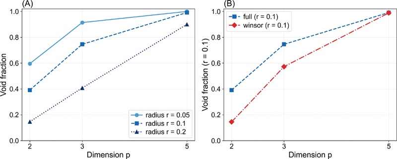
Void fraction of the physicochemical space as a function of dimensionality (p = 2, 3, 5). The void fraction is the proportion of random reference points in the min-max normalized space that lie farther than radius r from every sample. (A) Full data at three radii (r = 0.05, 0.1, 0.2). (B) Full data versus the winsorized version (top/bottom 1% clipped) at r = 0.1. N = 356.

최근접이웃거리

점 간 최근접이웃거리는 차원 증가에 따라 증가하였으며, 차원수에 따른 거리 증가를 √(차원수)로 보정한 후에도 증가 경향이 유지되었다(Fig. 5).

Fig. 5.

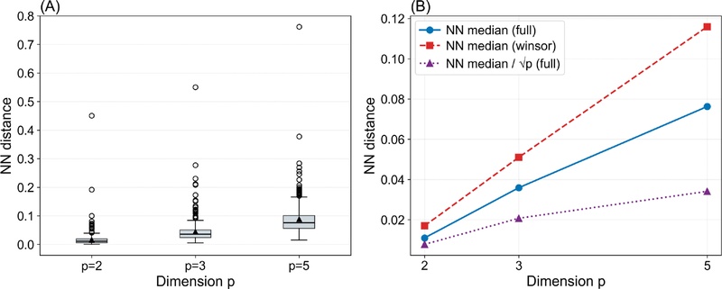
Nearest-neighbor (NN) distance in the min-max normalized space as a function of dimensionality (p = 2, 3, 5). (A) Distribution of per-point NN distances for the full data (boxplots; black triangles indicate the mean, open circles indicate outliers). (B) Median NN distance for the full and winsorized (top/bottom 1% clipped) data, together with the axis-corrected median (median / √p) for the full data. N = 356.

필요 표본수

동일 밀도의 충진에 필요한 표본수는 차원 증가에 따라 증가하여, 5차원에서는 추정 모집단 규모(국내 등록농약 농촌진흥청 농약안전정보시스템 2025년 6월 24일 기준)를 넘었다(Fig. 6).

Fig. 6.

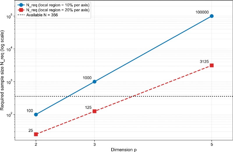
Required sample size (N_req) to place one point per local region as a function of dimensionality (p = 2, 3, 5), on a logarithmic scale, compared with the available sample (N = 356; dotted line). N_req is shown for local-region sizes of 10% and 20% per axis.

Void fraction과 필요한 표본수가 차원에 따라 급격히 증가한 양상은 차원의 저주로 알려진 현상과 부합하며, 차원이 늘수록 공간의 부피가 기하급수적으로 커지기 때문이다(Ronan et al., 2016). Space-filing 설계의 목표가 공간의 어느 지점에서도 가까운 설계점이 존재하도록 배치하는 데 있음을 고려하면(Joseph, 2016), 차원이 높아질수록 많은 표본이 필요해진다. 따라서 피부 투과성을 정의하는 5변수 공간을 균등하게 채우는데 필요한 표본수는 국내 등록 농약 원제 전체를 동원하여도 도달할 수 없는 규모이기 때문에 대표 선정은 이보다 낮은 차원의 축에서 수행되어야 한다. 표본을 늘려도 목표 수준에 도달하지 못하는 경우가 존재한다는 점은 다른 분야의 표집 설계 연구에서도 보고되어 있다(He et al., 2022).

아울러 커버리지 분석의 5 물성 변수가 실질적으로 서로 다른 축을 구성하는지 확인한 결과, log P와 수용해도만이 강한 음의 상관을 보였고(r = -0.81) 나머지 아홉 변수쌍은 모두 |r| < 0.56였다(Table 4). 모든 변수의 VIF가 5 미만(최대 4.40, 수용해도)으로 다중공선성은 관찰되지 않았다.

Table 4.

Pearson correlation matrix and variance inflation factors (VIF) among the five physicochemical variables

대표 물질 선정

log Kp 오분위 구간별로 log P·MW 평면상 최원점 선정을 수행하여 총 25종을 선정하였다(Fig. 7). 선정된 대표 물질의 log Kp 분포는 -6.62 ~ +0.06으로 5구간 전체를 포괄하였며, 물성값은 Table 5에 제시하였다.

Fig. 7.

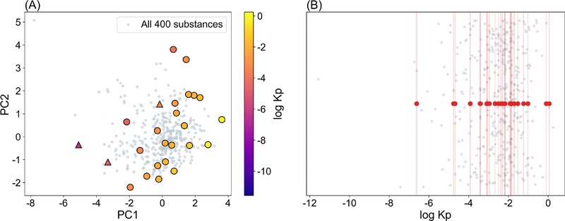
Coverage of the 25 selected representative compounds. (A) Principal component analysis (PCA) of the population in the log P-MW-log Kp space; gray points denote all 400 substances and the enlarged markers denote the 25 representatives, colored by log Kp. Circles indicate compounds retained from the initial farthest-point selection; triangles indicate compounds replaced by experimentally feasible substitutes within the same log Kp quintile. (B) Distribution of the 25 representatives (red points and vertical lines) along the log Kp axis, overlaid on the population (gray points).

Table 5.

Physicochemical properties of the 25 representative compounds selected by space-filling sampling across the five log Kp quintiles.

실험적으로 측정 불가능한 저투과 물질(거대분자 및 금속 착물 등)을 제외함에 따라 log Kp 하한이 -11.6에서 -6.6으로 상승하였으며, 이 영역은 모델의 외삽 한계로 명시하였다. 최원점 알고리즘은 결정적이므로 선정 결과는 시드에 무관하며, 실험 부적합 물질 교체 후에도 5구간 전체의 대표성과 물성 공간 분포가 유지되었다.

선정된 대표 25종의 커버리지 우수성은 무작위 선정과의 비교로 확인되었다(Fig. 8). log Kp 일차원 축에서 평균 커버 거리는 대표 선정이 0.0087로 무작위 추출 1,000회 평균(0.0114) 보다 낮았다. 최대 빈틈 또한 대표 선정이 0.4193로 무작위 평균(0.4959)보다 낮았다. 두 지표 모두 임의의 범위 절단 없이 극단 꼬리를 포함한 400종 전체에서 산출되었다.

Fig. 8.

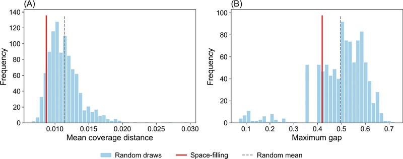
Coverage of the space-filling selection versus random selection along the log Kp axis, evaluated on the full population of 400 substances (including the extreme tails) in the min-max normalized [0,1] space. (A) Mean coverage distance and (B) maximum gap; for both metrics, lower values indicate better coverage. Histograms show the distribution over 1,000 random draws of 25 compounds (seed 42); the red solid line marks the space-filling selection and the gray dashed line marks the mean of the random draws.

종합하면, 국내 등록 농약 원제의 피부투과 관련 물성공간에 뚜렷한 군집 구조가 존재하지 않음을 다섯 가지 진단과 양성 및 음성 대조군을 통해 확인하였다. 또한, 군집이 부재한 연속 물성 공간에서 한정된 실측 자원을 배분하는 문제를 space-filling 표본 설계로 정식화하여, log Kp 오분위 구간을 포괄하는 25종의 대표 물질을 도출하였다. 무작위 선정과의 커버리지 비교를 통해 이 선정이 임의 추출보다 물성 스펙트럼을 더 균등하게 대표함을 확인하였다. 다만 선정이 log Kp 축에서 수행되었으므로 5변수 공간 전체에서의 균등성은 보장되지 않으며, 이는 표본이 확충된 이후의 과제로 남는다. 이 결과는 후속 동물대체 시험법의 실측 대상 선정 및 예측 모델 구축의 학습자료로 활용된다. 또한 분석에 사용된 농약의 물성은 다른 위해성 평가 분야에서도 공통적으로 이용되는 항목이므로, 군집 부재라는 진단 결과는 피부흡수 이외의 평가 영역에도 활용될 수 있다.

Acknowledgments

본 연구는 2026년 농촌진흥청 국립농업과학원 농업과학기술 연구개발사업 ‘피부흡수율 동물대체시험법 개발을 통한 농약노출 위해성평가기준 개선(PJ017781)’에서 지원받아 수행되었으며, 2026년도 농촌진흥청 국립농업과학원 전문연구원 과정 지원사업에 의해 이루어진 것입니다.

REFERENCES

• Adolfsson A, Ackerman M, Brownstein NC, 2019. To cluster, or not to cluster: an analysis of clusterability methods. Pattern Recognit. 88:13-26. [https://doi.org/10.1016/j.patcog.2018.10.026]
• Daszykowski M, Walczak B, Massart DL, 2002. Representative subset selection. Anal. Chim. Acta 468(1):91-103. [https://doi.org/10.1016/S0003-2670(02)00651-7]
• Eleftheriadou D, Luette S, Kneuer C, 2019. In silico prediction of dermal absorption of pesticides - an evaluation of selected models against results from in vitro testing. SAR QSAR Environ. Res. 30(8):561-585. [https://doi.org/10.1080/1062936X.2019.1644533]
• European Food Safety Authority (EFSA), 2017. Guidance on dermal absorption. EFSA J. 15(6):4873. [https://doi.org/10.2903/j.efsa.2017.4873]
• Golbraikh A, Tropsha A, 2002. Predictive QSAR modeling based on diversity sampling of experimental datasets for the training and test set selection. J. Comput.-Aided Mol. Des. 16(5-6):357-369. [https://doi.org/10.1023/A:1020869118689]
• Hartigan JA, Hartigan PM, 1985. The dip test of unimodality. Ann. Stat. 13(1):70-84. [https://doi.org/10.1214/aos/1176346577]
• He J, Zhou X, Matsui T, Li F, Tanaka TST, 2022. Critical reevaluation of an efficient sampling design for assessing soil properties using bootstrap sampling and geostatistical analysis in Japanese large-scale paddy fields. Soil Sci. Plant Nutr. 68(5-6):536-546. [https://doi.org/10.1080/00380768.2022.2101864]
• Hopkins B, Skellam JG, 1954. A new method for determining the type of distribution of plant individuals. Ann. Bot. 18(2):213-227. [https://doi.org/10.1093/oxfordjournals.aob.a083391]
• Hubert L, Arabie P, 1985. Comparing partitions. J. Classif. 2(1):193-218. [https://doi.org/10.1007/BF01908075]
• Joseph VR, 2016. Space-filling designs for computer experiments: a review. Qual. Eng. 28(1):28-35. [https://doi.org/10.1080/08982112.2015.1100447]
• Kalogeratos A, Likas A, 2012. Dip-means: an incremental clustering method for estimating the number of clusters. Adv. Neural Inf. Process. Syst. 25:2393-2401.
• Kar S, Amin SA, Li L, 2025. Unveiling chemical space, scaffold diversity, critical structural features of pesticides: a comprehensive QSAR, qRASAR, machine learning studies to predict pesticides toxicity. Sci. Total Environ. 1001:180489. [https://doi.org/10.1016/j.scitotenv.2025.180489]
• Kennard RW, Stone LA, 1969. Computer aided design of experiments. Technometrics 11(1):137-148. [https://doi.org/10.1080/00401706.1969.10490666]
• Kobak D, Linderman GC, 2021. Initialization is critical for preserving global data structure in both t-SNE and UMAP. Nat. Biotechnol. 39(2):156-157. [https://doi.org/10.1038/s41587-020-00809-z]
• Krieger RI, 1995. Pesticide exposure assessment. Toxicol. Lett. 82/83:65-72. [https://doi.org/10.1016/0378-4274(95)03545-1]
• Martin TM, Harten P, Young DM, Muratov EN, Golbraikh A, et al., 2012. Does rational selection of training and test sets improve the outcome of QSAR modeling? J. Chem. Inf. Model. 52(10):2570-2578. [https://doi.org/10.1021/ci300338w]
• McInnes L, Healy J, Melville J, 2018. UMAP: uniform manifold approximation and projection for dimension reduction. arXiv:1802.03426, . [https://doi.org/10.21105/joss.00861]
• Organisation for Economic Co-operation and Development (OECD), 2004. Guidance document for the conduct of skin absorption studies. Series on Testing and Assessment No. 28. Paris, France.
• Organisation for Economic Co-operation and Development (OECD), 2022. Guidance notes on dermal absorption. Series on Testing and Assessment No. 156, 2nd ed. Paris, France.
• Pedregosa F, Varoquaux G, Gramfort A, Michel V, Thirion B, et al., 2011. Scikit-learn: machine learning in Python. J. Mach. Learn. Res. 12:2825-2830.
• Potts RO, Guy RH, 1992. Predicting skin permeability. Pharm. Res. 9(5):663-669. [https://doi.org/10.1023/A:1015810312465]
• Renai L, Turkina V, Hulleman T, Nikolopoulos A, Gargano AFG, et al., 2025. A novel chemical-space-dependent strategy for compound selection in non-target LC-HRMS method development using physicochemical and structural data. Environ. Sci. Technol. Lett. 12(9):1162-1168. [https://doi.org/10.1021/acs.estlett.5c00759]
• Ronan T, Qi Z, Naegle KM, 2016. Avoiding common pitfalls when clustering biological data. Sci. Signal. 9(432):re6. [https://doi.org/10.1126/scisignal.aad1932]
• Rousseeuw PJ, 1987. Silhouettes: a graphical aid to the interpretation and validation of cluster analysis. J. Comput. Appl. Math. 20:53-65. [https://doi.org/10.1016/0377-0427(87)90125-7]
• Rural Development Administration (RDA), 2026. Registration criteria for pesticides and active ingredients. RDA Notification No. 2026-15, Annex 12. Jeonju, Korea. (In Korean)
• Wang B, Mezlini AM, Demir F, Fiume M, Tu Z, et al., 2014. Similarity network fusion for aggregating data types on a genomic scale. Nat. Methods 11(3):333-337. [https://doi.org/10.1038/nmeth.2810]
• Waters LJ, Quah XL, 2022. Predicting skin permeability using HuskinDB. Sci. Data 9:584. [https://doi.org/10.1038/s41597-022-01698-4]
• Wright K, 2022. Will the real Hopkins statistic please stand up? R J. 14(3):282-292. [https://doi.org/10.32614/RJ-2022-055]
• You AS, Lee N, Park S, Jo Y, Oh JA, et al., 2017. Estimation of exposure dose and occupational risk assessment with various dermal absorption default in spraying of plant protection products. Korean J. Pestic. Sci. 21(4):434-452. (In Korean) [https://doi.org/10.7585/kjps.2017.21.4.434]